demand and its elasticity

February 21, 2012

demand and its elasticity

Price elasticity of demand (PED or E_d) is a measure used in economics to show the responsiveness, or elasticity, of the quantity demanded of a good or service to a change in its price. More precisely, it gives the percentage change in quantity demanded in response to a one percent change in price (holding constant all the other determinants of demand, such as income). It was devised byAlfred Marshall.

Price elasticities are almost always negative, although analysts tend to ignore the sign even though this can lead to ambiguity. Only goods which do not conform to the law of demand, such as Veblenand Giffen goods, have a positive PED. In general, the demand for a good is said to be inelastic (or relatively inelastic) when the PED is less than one (in absolute value): that is, changes in price have a relatively small effect on the quantity of the good demanded. The demand for a good is said to be elastic (or relatively elastic) when its PED is greater than one (in absolute value): that is, changes in price have a relatively large effect on the quantity of a good demanded.

Revenue is maximized when price is set so that the PED is exactly one. The PED of a good can also be used to predict the incidence (or "burden") of a tax on that good. Various research methods are used to determine price elasticity, including test markets, analysis of historical sales data and conjoint analysis.

[hide]

[edit]Definition

PED is a measure of responsiveness of the quantity of a good or service demanded to changes in its price.^[1] The formula for the coefficient of price elasticity of demand for a good is:^[2]^[3]^[4]

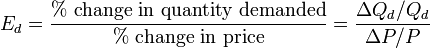
$E_d = \frac{\%\ \mbox{change in quantity demanded}}{\%\ \mbox{change in price}} = \frac{\Delta Q_d/Q_d}{\Delta P/P}$

The above formula usually yields a negative value, due to the inverse nature of the relationship between price and quantity demanded, as described by the "law of demand".^[3] For example, if the price increases by 5% and quantity demanded decreases by 5%, then the elasticity at the initial price and quantity = −5%/5% = −1. The only classes of goods which have a PED of greater than 0 areVeblen and Giffen goods.^[5] Because the PED is negative for the vast majority of goods and services, however, economists often refer to price elasticity of demand as a positive value (i.e., in absolute value terms).^[4]

This measure of elasticity is sometimes referred to as the own-price elasticity of demand for a good, i.e., the elasticity of demand with respect to the good's own price, in order to distinguish it from the elasticity of demand for that good with respect to the change in the price of some other good, i.e., a complementary or substitute good.^[1] The latter type of elasticity measure is called a cross-price elasticity of demand.^[6]^[7]

As the difference between the two prices or quantities increases, the accuracy of the PED given by the formula above decreases for a combination of two reasons. First, the PED for a good is not necessarily constant; as explained below, PED can vary at different points along the demand curve, due to its percentage nature.^[8]^[9] Elasticity is not the same thing as the slope of the demand curve, which is dependent on the units used for both price and quantity.^[10]^[11] Second, percentage changes are not symmetric; instead, the percentage change between any two values depends on which one is chosen as the starting value and which as the ending value. For example, if quantity demanded increases from 10 units to 15 units, the percentage change is 50%, i.e., (15 − 10) ÷ 10 (converted to a percentage). But if quantity demanded decreases from 15 units to 10 units, the percentage change is −33.3%, i.e., (10 − 15) ÷ 15.^[12]^[13]

Two alternative elasticity measures avoid or minimise these shortcomings of the basic elasticity formula: point-price elasticity and arc elasticity.

[edit]Point-price elasticity

One way to avoid the accuracy problem described above is to minimise the difference between the starting and ending prices and quantities. This is the approach taken in the definition of point-priceelasticity, which uses differential calculus to calculate the elasticity for an infinitesimal change in price and quantity at any given point on the demand curve: ^[14]

$E_d = \frac{P}{Q_d}\times\frac{dQ_d}{dP}$

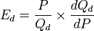
In other words, it is equal to the absolute value of the first derivative of quantity with respect to price (dQ_d/dP) multiplied by the point's price (P) divided by its quantity (Q_d).^[15]

In terms of partial-differential calculus, point-price elasticity of demand can be defined as follows:^[16] let $\displaystyle x(p,w)$ be the demand of goods $x_1,x_2,\dots,x_L$ as a function of parameters price and wealth, and let $\displaystyle x_l(p,w)$ be the demand for good $\displaystyle l$ . The elasticity of demand for good $\displaystyle x_l(p,w)$ with respect to price

p k

$E_{x_l,p_k} = \frac{\partial x_l(p,w)}{\partial p_k}\cdot\frac{p_k}{x_l(p,w)} = \frac{\partial \log x_l(p,w)}{\partial \log p_k}$

However, the point-price elasticity can be computed only if the formula for the demand function,

Q d = f (P)

, is known so its derivative with respect to price,

d Q d / d P

, can be determined.

[edit]Arc elasticity

A second solution to the asymmetry problem of having a PED dependent on which of the two given points on a demand curve is chosen as the "original" point and which as the "new" one is to compute the percentage change in P and Q relative to the average of the two prices and the average of the two quantities, rather than just the change relative to one point or the other. Loosely speaking, this gives an "average" elasticity for the section of the actual demand curve—i.e., the arc of the curve—between the two points. As a result, this measure is known as the arc elasticity, in this case with respect to the price of the good. The arc elasticity is defined mathematically as:^[13]^[17]^[18]

$E_d = \frac{\frac{P_1 + P_2}{2}}{\frac{Q_{d_1} + Q_{d_2}}{2}}\times\frac{\Delta Q_d}{\Delta P} = \frac{P_1 + P_2}{Q_{d_1} + Q_{d_2}}\times\frac{\Delta Q_d}{\Delta P}$

This method for computing the price elasticity is also known as the "midpoints formula", because the average price and average quantity are the coordinates of the midpoint of the straight line between the two given points.^[12]^[18] However, because this formula implicitly assumes the section of the demand curve between those points is linear, the greater the curvature of the actual demand curve is over that range, the worse this approximation of its elasticity will be.^[17]^[19]

[edit]History

The illustration that accompanied Marshall's original definition of PED, the ratio of PT to Pt

Together with the concept of an economic "elasticity" coefficient, Alfred Marshall is credited with defining PED ("elasticity of demand") in his book Principles of Economics, published in 1890.^[20] He described it thus: "And we may say generally:— the elasticity (or responsiveness) of demand in a market is great or small according as the amount demanded increases much or little for a given fall in price, and diminishes much or little for a given rise in price".^[21] He reasons this since "the only universal law as to a person's desire for a commodity is that it diminishes... but this diminution may be slow or rapid. If it is slow... a small fall in price will cause a comparatively large increase in his purchases. But if it is rapid, a small fall in price will cause only a very small increase in his purchases. In the former case... the elasticity of his wants, we may say, is great. In the latter case... the elasticity of his demand is small."^[22] Mathematically, the Marshallian PED was based on a point-price definition, using differential calculus to calculate elasticities.^[23]

[edit]Determinants

The overriding factor in determining PED is the willingness and ability of consumers after a price change to postpone immediate consumption decisions concerning the good and to search for substitutes ("wait and look").^[24] A number of factors can thus affect the elasticity of demand for a good:^[25]

Availability of substitute goods: the more and closer the substitutes available, the higher the elasticity is likely to be, as people can easily switch from one good to another if an even minor price change is made;^[25]^[26]^[27] There is a strong substitution effect.^[28] If no close substitutes are available the substitution of effect will be small and the demand inelastic.^[28]
- Breadth of definition of a good: the broader the definition of a good (or service), the lower the elasticity. For example, Company X's fish and chips would tend to have a relatively high elasticity of demand if a significant number of substitutes are available, whereas food in general would have an extremely low elasticity of demand because no substitutes exist.^[29]
Percentage of income: the higher the percentage of the consumer's income that the product's price represents, the higher the elasticity tends to be, as people will pay more attention when purchasing the good because of its cost;^[25]^[26] The income effect is substantial.^[30] When the goods represent only a negligible portion of the budget the income effect will be insignificant and demand inelastic,^[30]
Necessity: the more necessary a good is, the lower the elasticity, as people will attempt to buy it no matter the price, such as the case of insulin for those that need it.^[10]^[26]
Duration: for most goods, the longer a price change holds, the higher the elasticity is likely to be, as more and more consumers find they have the time and inclination to search for substitutes.^[25]^[27] When fuel prices increase suddenly, for instance, consumers may still fill up their empty tanks in the short run, but when prices remain high over several years, more consumers will reduce their demand for fuel by switching to carpooling or public transportation, investing in vehicles with greater fuel economy or taking other measures.^[26] This does not hold for consumer durables such as the cars themselves, however; eventually, it may become necessary for consumers to replace their present cars, so one would expect demand to be less elastic.^[26]
Brand loyalty: an attachment to a certain brand—either out of tradition or because of proprietary barriers—can override sensitivity to price changes, resulting in more inelastic demand.^[29]^[31]
Who pays: where the purchaser does not directly pay for the good they consume, such as with corporate expense accounts, demand is likely to be more inelastic.^[31]

[edit]Interpreting values of price elasticity coefficients

Perfectly inelastic demand^[10]

Perfectly elastic demand^[10]

Elasticities of demand are interpreted as follows:^[10]

Value	Descriptive Terms
E_d = 0	Perfectly inelastic demand
- 1 < E_d < 0	Inelastic or relatively inelastic demand
E_d = - 1	Unit elastic, unit elasticity, unitary elasticity, or unitarily elastic demand
- ∞ < E_d < - 1	Elastic or relatively elastic demand
E_d = - ∞	Perfectly elastic demand

A decrease in the price of a good normally results in an increase in the quantity demanded by consumers because of the law of demand, and conversely, quantity demanded decreases when price rises. As summarized in the table above, the PED for a good or service is referred to by different descriptive terms depending on whether the elasticity coefficient is greater than, equal to, or less than −1. That is, the demand for a good is called:

relatively inelastic when the percentage change in quantity demanded is less than the percentage change in price (so that E_d > - 1);
unit elastic, unit elasticity, unitary elasticity, or unitarily elastic demand when the percentage change in quantity demanded is equal to the percentage change in price (so that E_d = - 1); and
relatively elastic when the percentage change in quantity demanded is greater than the percentage change in price (so that E_d < - 1).^[10]

As the two accompanying diagrams show, perfectly elastic demand is represented graphically as a horizontal line, and perfectly inelastic demand as a vertical line. These are the only cases in which the PED and the slope of the demand curve (∆P/∆Q) are both constant, as well as the only cases in which the PED is determined solely by the slope of the demand curve (or more precisely, by the inverse of that slope).^[10]

[edit]Effect on total revenue

[edit]Effect on tax incidence

When demand is more inelastic than supply, consumers will bear a greater proportion of the tax burden than producers will.

Main article: tax incidence

PEDs, in combination with price elasticity of supply (PES), can be used to assess where the incidence (or "burden") of a per-unit tax is falling or to predict where it will fall if the tax is imposed. For example, when demand is perfectly inelastic, by definition consumers have no alternative to purchasing the good or service if the price increases, so the quantity demanded would remain constant. Hence, suppliers can increase the price by the full amount of the tax, and the consumer would end up paying the entirety. In the opposite case, when demand is perfectly elastic, by definition consumers have an infinite ability to switch to alternatives if the price increases, so they would stop buying the good or service in question completely—quantity demanded would fall to zero. As a result, firms cannot pass on any part of the tax by raising prices, so they would be forced to pay all of it themselves.^[36]

In practice, demand is likely to be only relatively elastic or relatively inelastic, that is, somewhere between the extreme cases of perfect elasticity or inelasticity. More generally, then, the higher the elasticity of demand compared to PES, the heavier the burden on producers; conversely, the more inelasticthe demand compared to PES, the heavier the burden on consumers. The general principle is that the party (i.e., consumers or producers) that has feweropportunities to avoid the tax by switching to alternatives will bear the greater proportion of the tax burden.^[36]In the end the whole tax burden is carried by individual households since they are the ultimate owners of the means of production that the firm utilises (see Circular flow of income).

[edit]Selected price elasticities

Various research methods are used to calculate price elasticities in real life, including analysis of historic sales data, both public and private, and use of present-day surveys of customers' preferences to build up test markets capable of modelling such changes. Alternatively, conjoint analysis (a ranking of users' preferences which can then be statistically analysed) may be used.^[37]

Though PEDs for most demand schedules vary depending on price, they can be modeled assuming constant elasticity.^[38] Using this method, the PEDs for various goods—intended to act as examples of the theory described above—are as follows. For suggestions on why these goods and services may have the PED shown, see the above section on determinants of price elasticity.

Cigarettes (US)^[39]
- −0.3 to −0.6 (General)
- −0.6 to −0.7 (Youth)
Alcoholic beverages (US)^[40]
- −0.3 or −0.7 to −0.9 as of 1972 (Beer)
- −1.0 (Wine)
- −1.5 (Spirits)
Airline travel (US)^[41]
- −0.3 (First Class)
- −0.9 (Discount)
- −1.5 (for Pleasure Travelers)
Livestock
- −0.5 to −0.6 (Broiler Chickens)^[42]
Oil (World)
- −0.4
Car fuel^[43]
- −0.09 (Short run)
- −0.31 (Long run)
Medicine (US)
- −0.31 (Medical insurance)^[44]
- −.03 to −.06 (Pediatric Visits)^[45]

Rice^[46]
- −0.47 (Austria)
- −0.8 (Bangladesh)
- −0.8 (China)
- −0.25 (Japan)
- −0.55 (US)
Cinema visits (US)
- −0.87 (General)^[44]
Live Performing Arts (Theater, etc.)
- −0.4 to −0.9^[47]
Transport
- −0.20 (Bus travel US)^[44]
- −2.8 (Ford compact automobile)^[48]
Soft drinks
- −0.8 to −1.0 (general)^[49]
- −3.8 (Coca-Cola)^[50]
- −4.4 (Mountain Dew)^[50]
Steel
- −0.2 to −0.3^[51]
Eggs
- −0.1 (US: Household only),^[52] −0.35 (Canada),^[53] −0.55 (South Africa)^[54]